installer guru - Excel formating & conditional formating functions
Excel Formatting & Conditional Formatting Functions | Step-by-Step Guide
Excel Formatting & Conditional Formatting Functions
Learn how to make your Excel sheets look professional using basic formatting and powerful conditional formatting. We’ll use simple student marks data with step-by-step visuals and a Hindi video tutorial.
🎥 Video Tutorial – Excel Formatting & Conditional Formatting
Watch this full lesson from Installer Guru:
📂 Sample Data Used
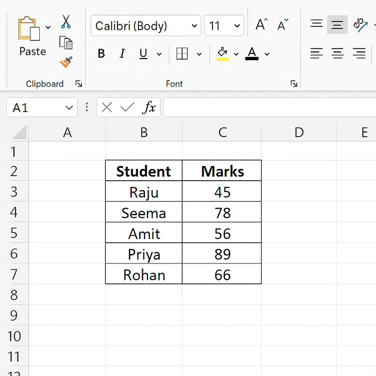
We’ll use the same student marks data as previous parts:
| Student | Marks |
|---|---|
| Raju | 45 |
| Seema | 78 |
| Amit | 56 |
| Priya | 89 |
| Rohan | 66 |
This data is entered in cells A2:B6 in Excel.
Step 1 – Basic Excel Formatting
1.1 Make Headers Bold
- Select cells A1:B1.
- On the Home tab, click the B icon (Bold).
1.2 Adjust Alignment
- Select cells B2:B6.
- Click Center alignment in the Alignment group.
1.3 Add Borders
- Select the range A1:B6.
- Click the Borders icon → choose All Borders.
These simple changes already make your sheet more readable and professional.
Step 2 – Font Color & Cell Fill Color
2.1 Add Header Background Color
- Select A1:B1.
- Click the Fill Color bucket and choose a light grey or any theme color.
- Optionally, change the font color to White and keep it Bold.
2.2 Color Code Important Marks Manually
- Select marks < 50 (e.g., B2 = 45) → set font color Red.
- Select high marks ≥ 80 (e.g., B4 = 89) → set cell fill color Green.
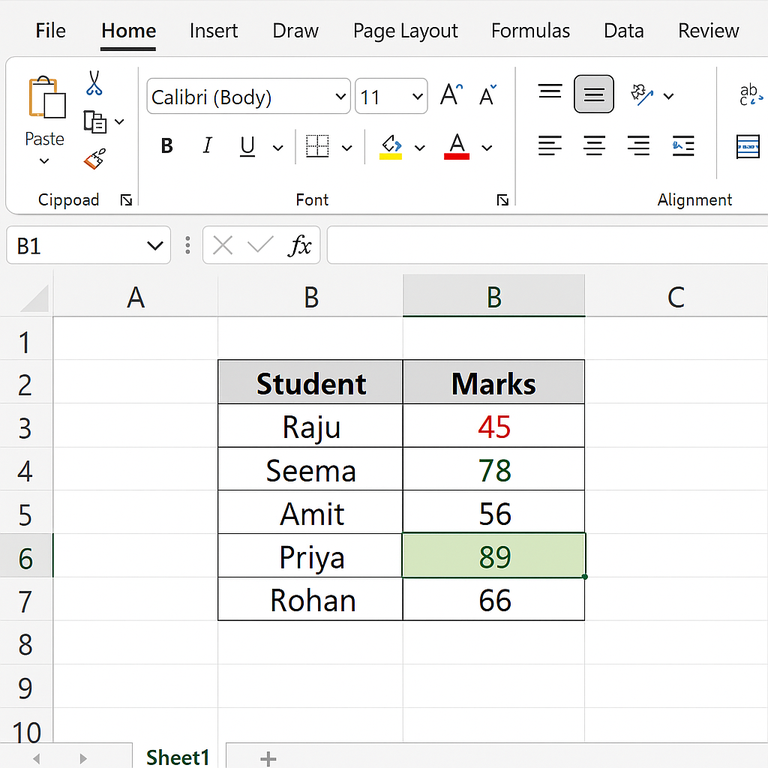
Manual formatting is useful for small data, but for larger tables we use Conditional Formatting.
Step 3 – Conditional Formatting: Highlight Marks > 60
3.1 What is Conditional Formatting?
Conditional Formatting automatically changes cell color, font, or style based on conditions you define (e.g., marks greater than 60).
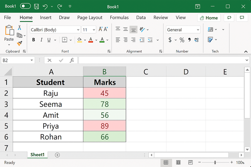
3.2 Create a Rule to Highlight Marks > 60
- Select the marks range B2:B6.
- Go to Home > Conditional Formatting > Highlight Cells Rules > Greater Than…
- In the box, type 60.
- Choose a format (for example, Light Green Fill with Dark Green Text).
- Click OK.
Now all marks higher than 60 (78, 89, 66) will automatically appear highlighted.
Step 4 – Conditional Formatting: Color Scales
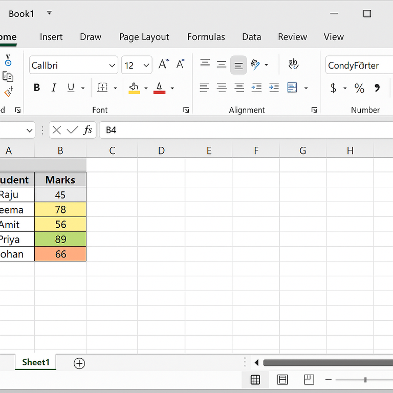
4.1 Apply a 3-Color Scale
- Select B2:B6 again.
- Go to Home > Conditional Formatting > Color Scales.
- Choose a 3-color scale (e.g., Red-Yellow-Green).
Excel will automatically color lower marks in red, middle values in yellow, and higher marks in green. This gives a quick visual idea of performance.
🧾 Summary of What You Learned
- Basic formatting: bold, alignment, borders.
- Font color and cell fill color for highlighting key data.
- Conditional Formatting to highlight marks > 60.
- Color scales to visualize low, medium, and high values instantly.
Combine these techniques to create clean, professional Excel reports for marks, sales, expenses, attendance, and more.
📌 Final Note
For a full demonstration in Hindi, watch the video tutorial above from Installer Guru and practice on your own Excel sheet.
Congratulations! You can now enjoy hassle-free invoicing with #InstallerGuru – Installation made easy.
Installer Guru
🚀 Installer Guru: Where Installation is Made Easy! 🌐💡 Join our community for simplified tech solutions, seamless installations, and a journey toward digital empowerment. Subscribe now and let's make technology easy, together! 🔧💻 #InstallationMadeEasy #installerguru
good